Hello! this is Jooyoung Kim, an engineer and music producer.
Today, I’d like to explain Spinorama, a concept anyone interested in sound and speakers should know. Let’s get started!
First, let’s briefly look at the history of how Spinorama measurements were developed.
Spinorama was created in the 1980s by Dr. Floyd Toole, a leading authority on speaker acoustics, while he was working at the National Research Council of Canada. In the 1990s, it was further refined in collaboration with Harman International. It has since been incorporated into standards issued by the American National Standards Institute (ANSI) and the Consumer Electronics Association (CEA).
Standard Method Of Measurement For In-Home Loudspeakers
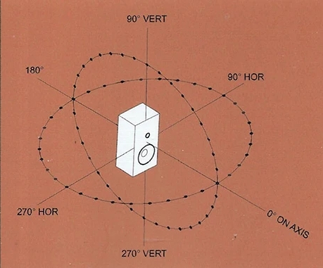
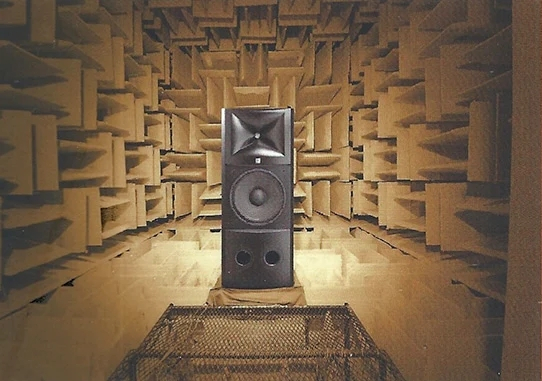
The measurement process, as shown above, involves taking measurements every 10 degrees horizontally and vertically in an anechoic chamber, resulting in a total of 70 data points.
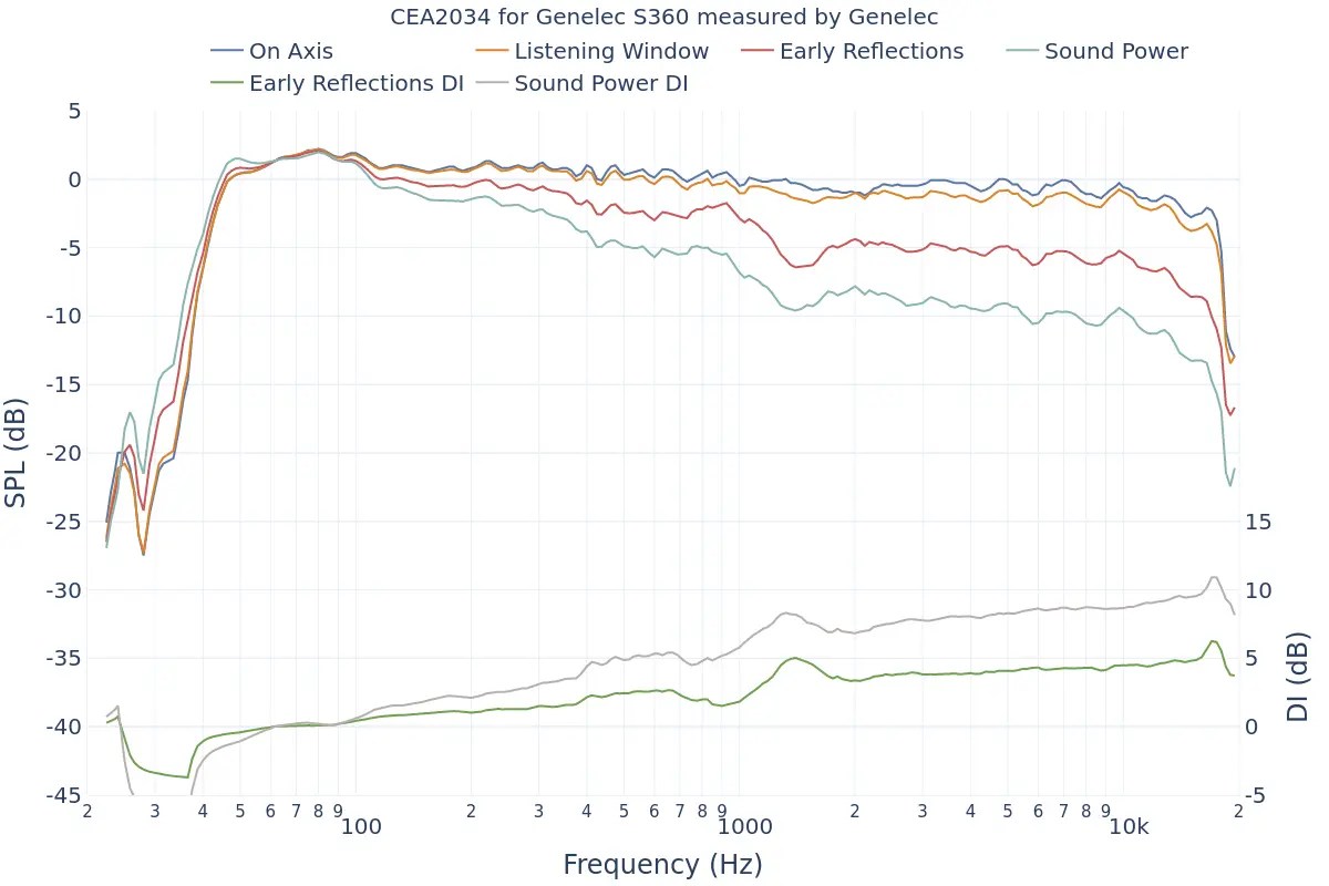
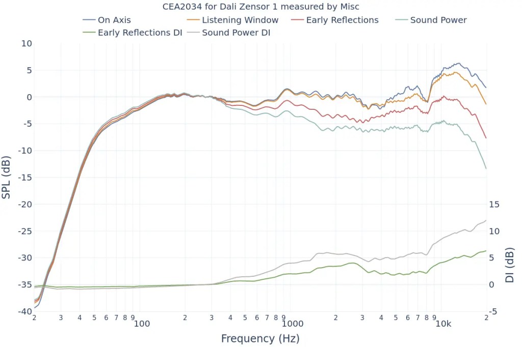
The collected data is represented in six frequency response graphs known as Spinorama charts.

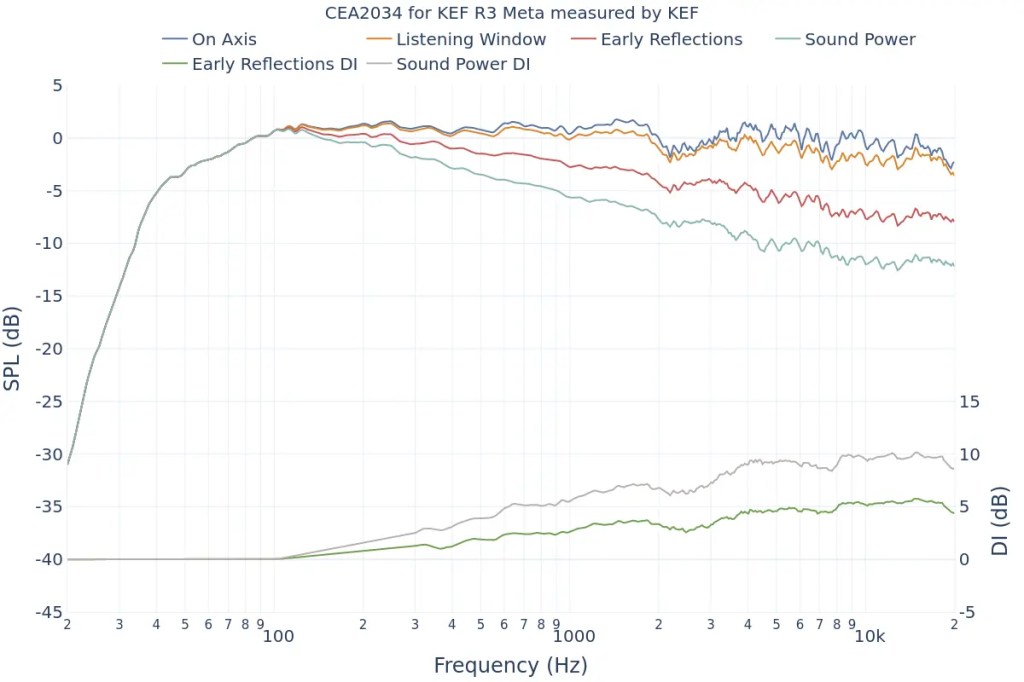
Let’s look at the Spinorama graph for my recently purchased KEF R3 META. The vertical axis is dB SPL (the unit we often use to measure sound levels, like airplane noise), and the horizontal axis is Hz (the unit of frequency).
- The top blue line is the On Axis response, representing the frequency response directly in front of the speaker. Manufacturers commonly provide this graph, but it lacks comprehensive information.
- The second orange line is the Listening Window response, which averages the frequency responses from ±10 degrees vertically and ±30 degrees horizontally, totaling 9 measurements. This approximates the expected response in a typical listening environment.
- The third red line represents Early Reflections, showing the response of early reflected sounds. It averages 8 measurements taken at ±40, ±60, and ±80 degrees horizontally, and ±50 degrees vertically. A significant difference from the On Axis and Listening Window responses helps distinguish between direct and reflected sounds.
- The light blue Sound Power response averages all 70 measurements. The more this graph parallels the other graphs without significant fluctuations, the better the speaker’s acoustic performance.
- The green Early Reflections DI (Directivity Index) is the difference between the On Axis and Early Reflections responses. This graph helps to quickly understand the difference between direct and reflected sounds.
- The brown Sound Power DI is the difference between the On Axis and Sound Power responses. Research suggests that smoother changes in both DI graphs are preferred by listeners (I’d provide the exact study, but finding it would take some time… I’ll update if I come across it later).
- The On Axis chart shows the basic frequency response.
- The closer the Listening Window response is to the On Axis response, the more similar the sound will be for the listener and those around them. This indicates good off-axis performance, meaning the sound remains consistent even if the listener moves slightly.
- The more aligned the Early Reflections, Sound Power, and On Axis graphs are, the higher the preference among listeners. If it’s hard to judge, check the DI graphs for a consistent slope.
This gives a basic understanding of Spinorama charts.
Of course, Spinorama charts have their limitations. As the title suggests, you shouldn’t choose a speaker based solely on these charts. However, they are a fundamental indicator for understanding a speaker’s performance, making them valuable knowledge for anyone in music or sound.
In future posts, I’ll discuss near-field measurements by the German company Klippel.
Finally,
This site offers Spinorama charts for many speakers measured so far. Since it aggregates data from various sources, make sure to choose highly reliable sources in the settings tab for accurate information.
I hope this post is helpful for you! See you in the next post!
