Manley Nu Mu Stereo Limiter/Compressor Review

Hello! This is Jooyoung Kim, an audio engineer and music producer.

Now that the semester is over, I have a few weeks to rest and prepare materials for my next classes. Even so, I still have a lot of work to do on my new research, my DIY hardware projects, and my English studies. It will be very busy holidays.


By the way, recently, I decided that I need to sell my compressors, the Heritage Audio Successor and the Stam Audio SA-4000 MK2, and replace them with a mastering-grade compressor to mix and master music better.

Fortunately, last week I sold both of them, and I have been happily considering which mastering-grade compressor I should buy. There were several options to choose from, but I finally decided to buy the Manley Nu Mu Stereo Limiter/Compressor.

This decision came from my experience with the SPL IRON, the SPL Venos, and the Chandler Limited RS660 compressors, which are vari-mu-style compressors. They sound great across many genres, but they aren’t within my budget. (If I bought them, I’d have to live on cup noodles for about three months! :))

I also had an experience with the original Neve 33609/C compressor/limiter and the Chandler Limited EMI TG12413 Zener Limiter. These are diode-bridge compressors that have really great saturation; however, they are also unaffordable.

I found two reasonably priced compressors: the Rupert Neve Designs 5254 Shelford Diode Bridge Compressor and the Manley Nu Mu Stereo Limiter/Compressor. I ultimately chose the Manley because it was more affordable. Also, having previously owned a diode-bridge compressor—the Heritage Audio Successor—I was ready to explore a different style.

I was also attracted to the WesAudio ngBusComp, which features a handy digital recall system. However, it is a VCA-style compressor, which is the same type as the Stam Audio SA-4000 MK2 that I used to own.

Therefore, I decided to buy the Manley Nu Mu Stereo Limiter/Compressor!


Build Features

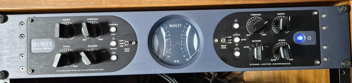
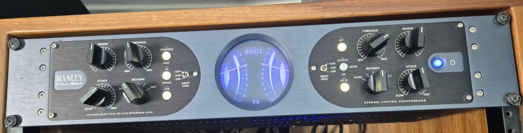
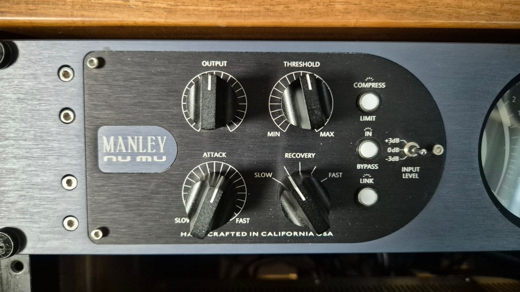
The Manley Nu Mu features eight knobs, six buttons, and two switches, excluding the power switch. The knobs (Threshold, Output, Recovery (Release), and Attack) and switches (Input Level) on the left side are identical to those on the right, allowing for independent adjustment of the left and right signals.

The Link button couples the left and right signal control knobs, with the notable exception of the Output controls. Consequently, these must be matched manually via measurement. Furthermore, apart from the Recovery knob, all controls feature continuous rotation, which makes precise recall of previous settings difficult.

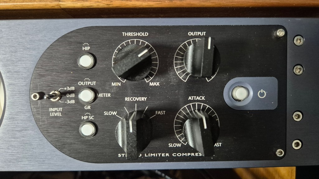
The HIP (High Impact Preservation) control compresses quieter sounds while leaving loud peaks untouched. It processes these signals internally to achieve results similar to parallel compression. I found that the audio sounds more natural when engaged, so I may leave this button on permanently.

The HP SC (Sidechain High Pass Filter) button activates an internal filter with a 100Hz corner frequency and a 6dB/octave slope. This prevents the compressor from reacting to low-frequency energy below 100Hz, ensuring more stable gain reduction.


Measurments

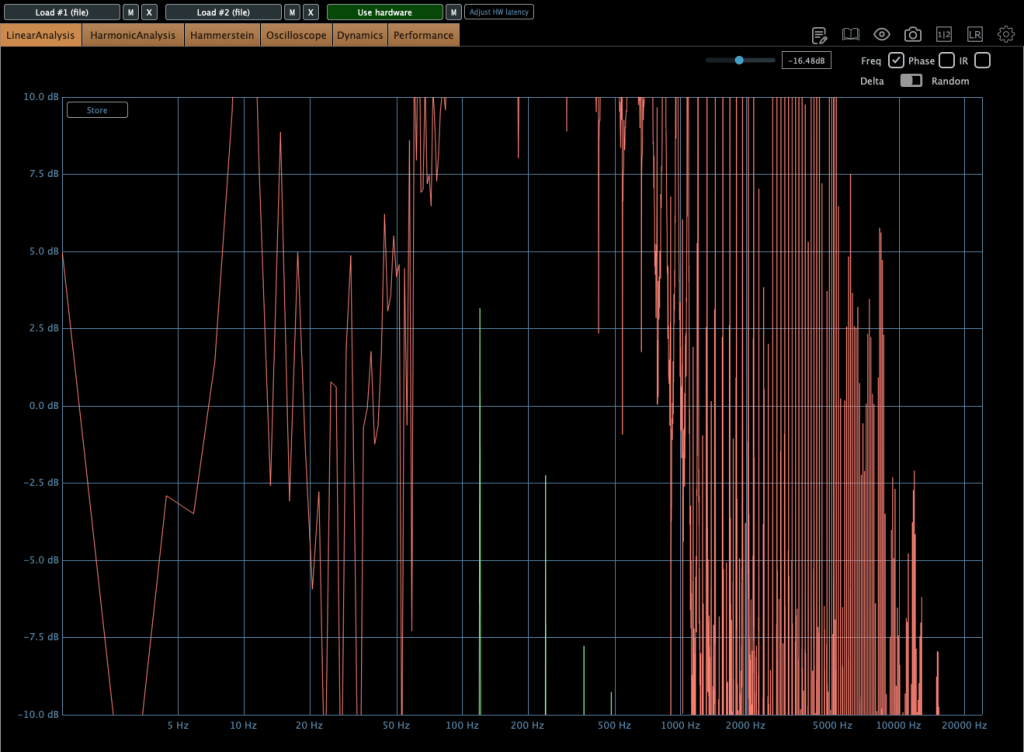
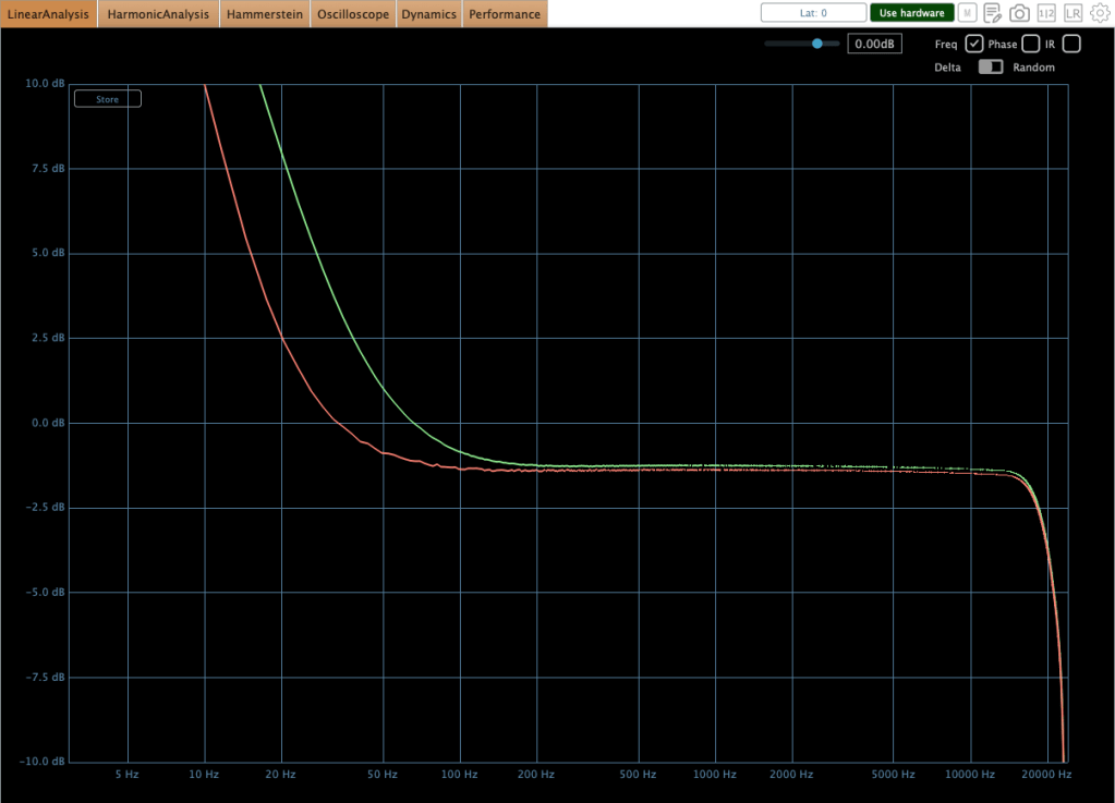
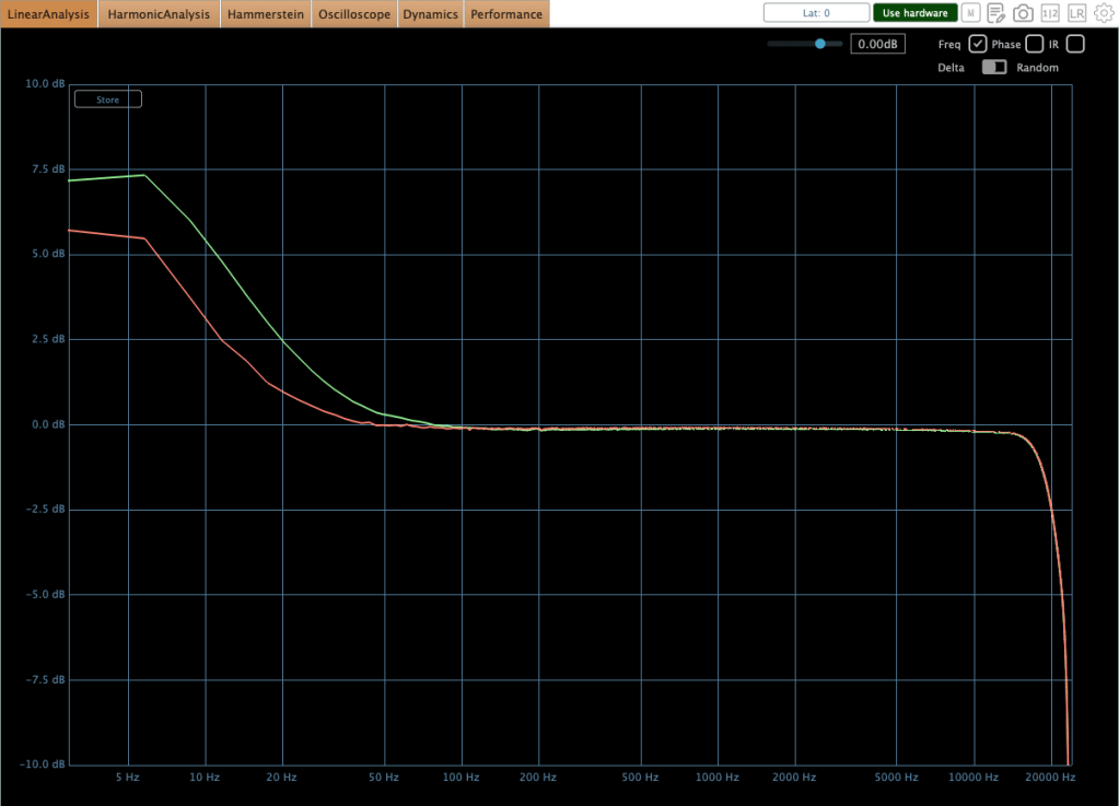
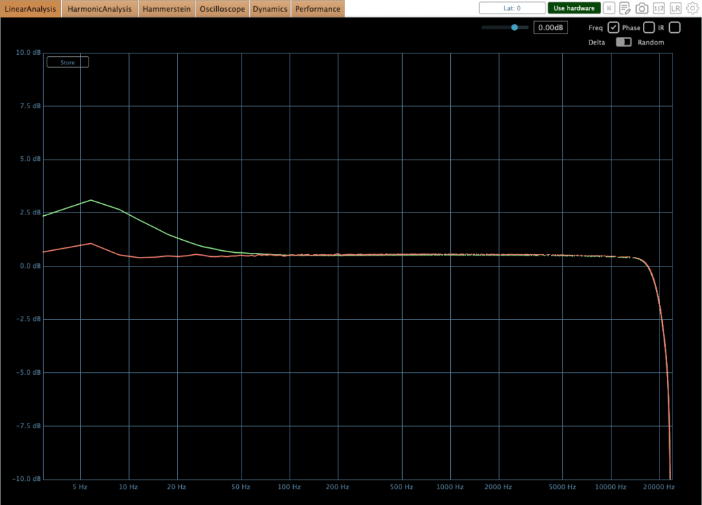
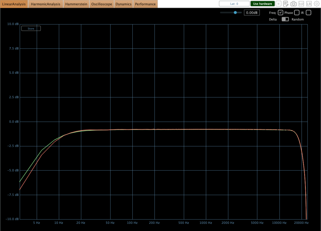
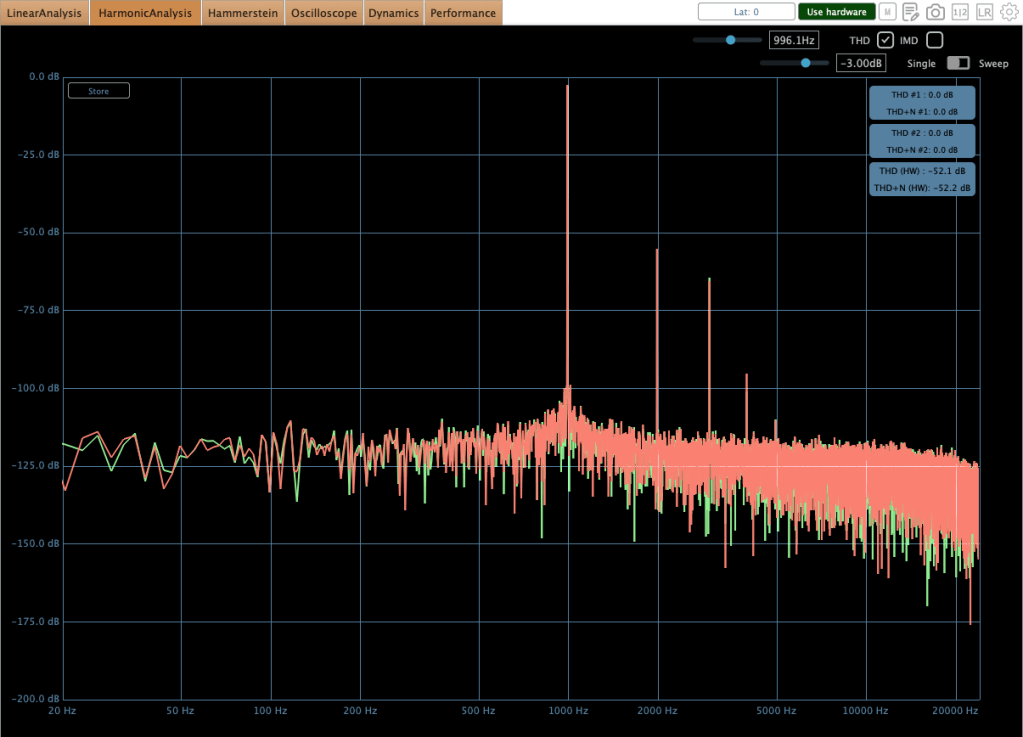
This equipment exhibits characteristic behaviors. Variations in input gain, threshold, attack time, and release time significantly affect the low-frequency response. Additionally, there is a slight amplitude discrepancy between the left and right circuits in the low end. This difference is easily observed in many compressors that do not naturally exhibit a low cut in their frequency response. For instance, when I demoed the SPL Venos, I found a significant discrepancy in the low-frequency output. Furthermore, an engineer peer of mine mentioned struggling with the same low-end inconsistency after purchasing an SPL Iron.

So, this level of discrepancy is acceptable.

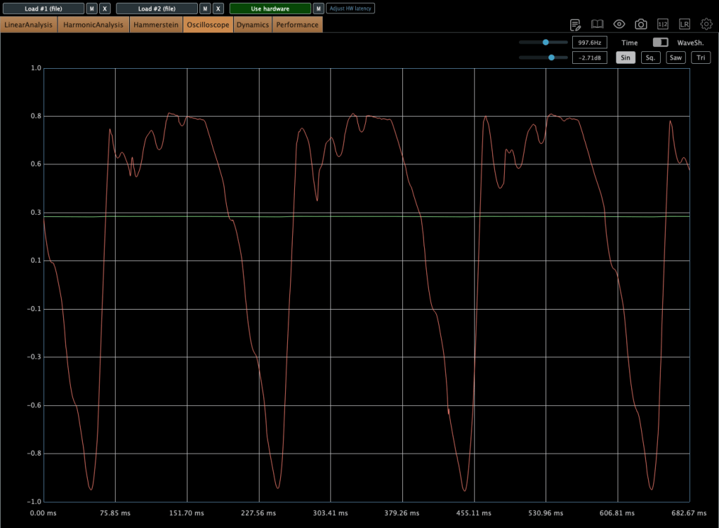
As shown in the image above, harmonic distortion levels are relatively low; however, they remain sufficient to noticeably alter the timbre of the sound.

Compressor mode
Limiter mode

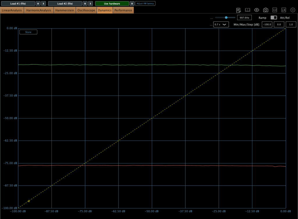
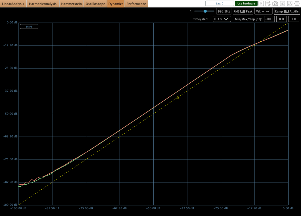
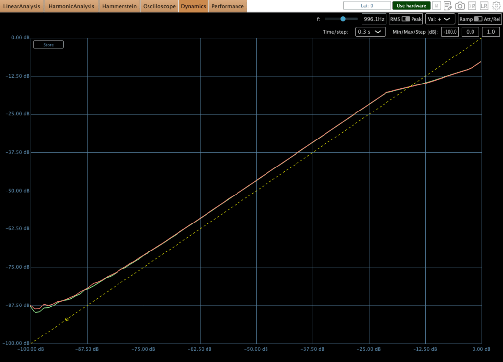
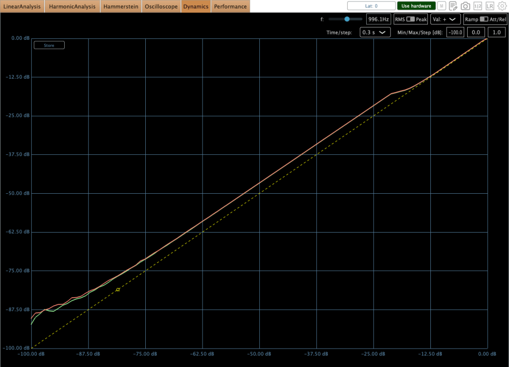
Regarding the compression curves, the unit provides a smooth transition in both modes; however, the Limiter mode utilizes a hard knee, whereas the Compressor mode employs a soft knee.

Compressor mode
Limiter mode

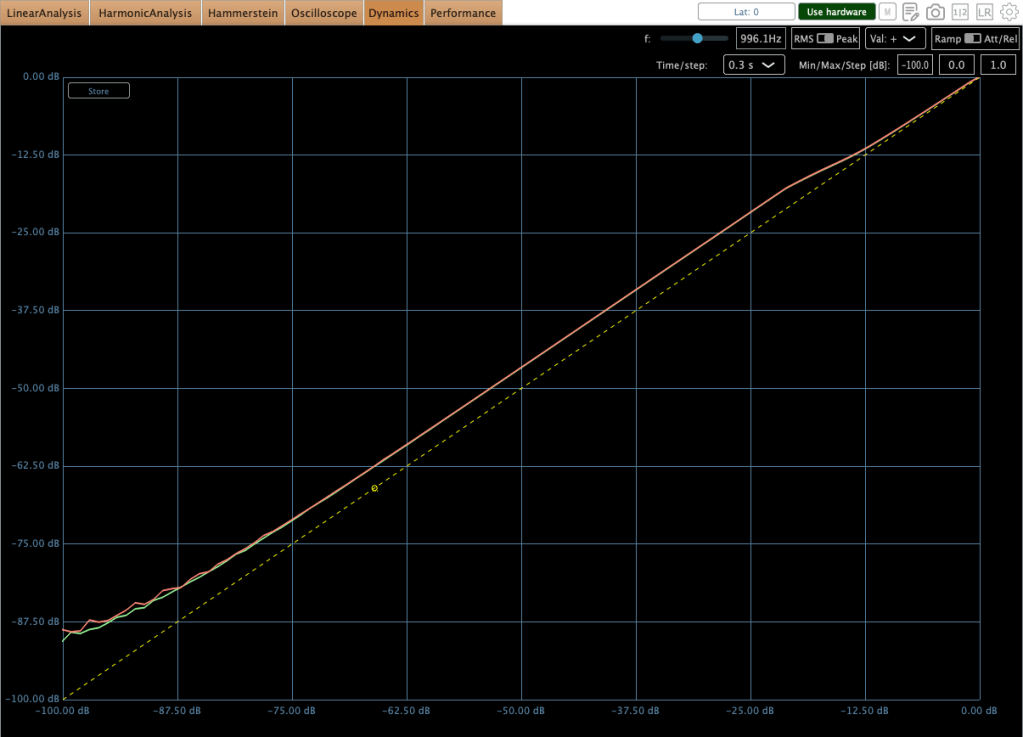
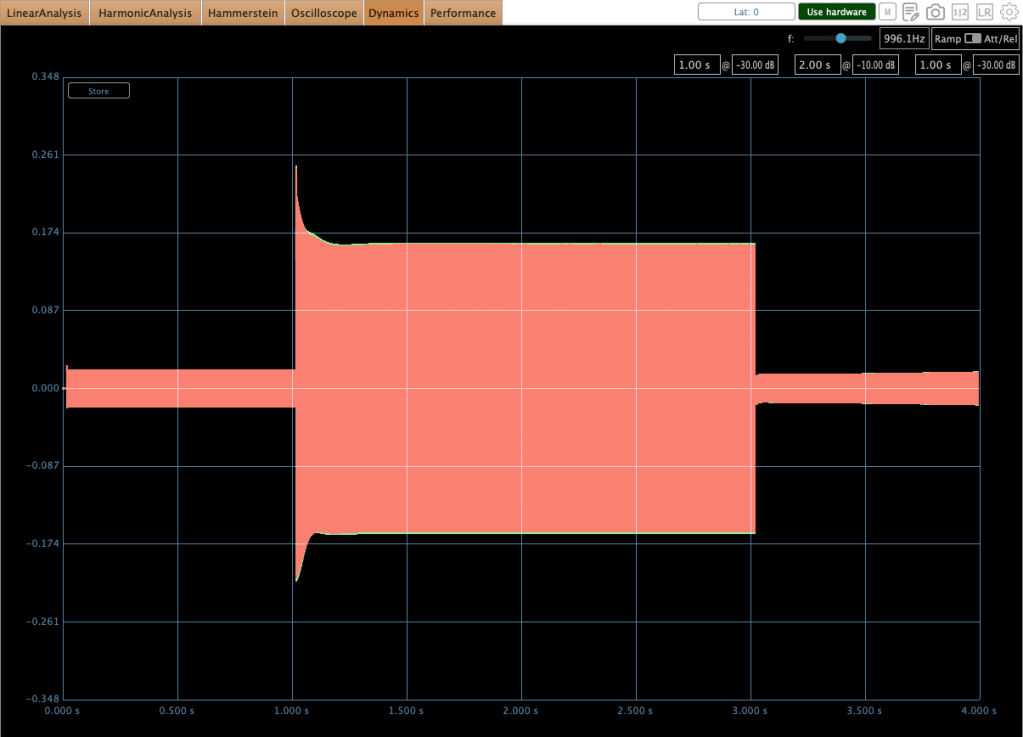
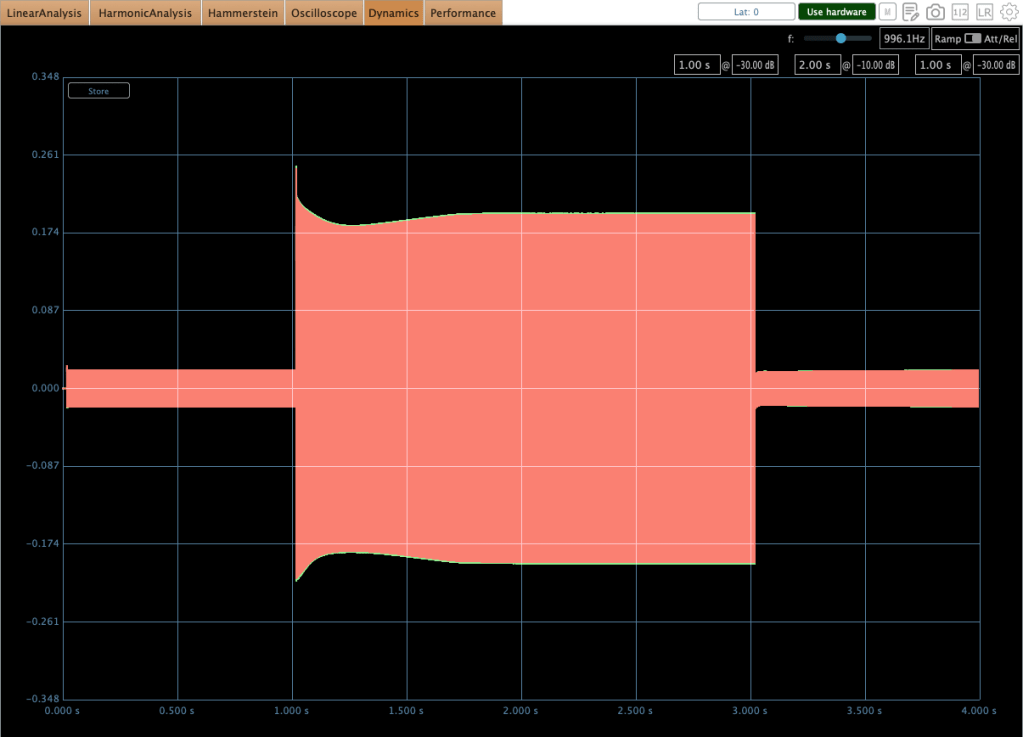
The images above illustrate the behavior of the unit in HIP mode

GR 2-3 dB
GR 1-2 dB

Furthermore, some peculiar behaviors occur during operation. Engineers typically target 0–2 dB of gain reduction on a mastering or mix bus compressor to achieve effective ‘glue.’ However, in this range, audible ‘pumping’ occurs. You can observe this specific behavior in the second photo above.

I encountered numerous discussions regarding this issue while researching the compressor prior to purchase. Although I anticipated the behavior, the audible effect was more critical than I had expected upon testing it myself.

Ultimately, I realized that the 0–2 dB gain reduction range is not ideal for this unit. Interestingly, pushing the gain reduction to 2–3 dB yields much better results, where the behavior stabilizes significantly in both compressor and limiter modes. This performance difference is illustrated in the first photo above.

It has a great sonic taste! It adds rich saturation and harmonic distortion across all frequency ranges, which fills out the empty spaces within the stereo field—a quality that is clearly audible.

However, because the character is so flavorful, I believe that applying a stereo imaging processor will help ‘release’ the sound that has become dense from the harmonic distortion, resulting in a more open and balanced result for mixing or mastering. To this end, I am looking forward to acquiring either an SPL Vitalizer MK3 or a Big Studio.

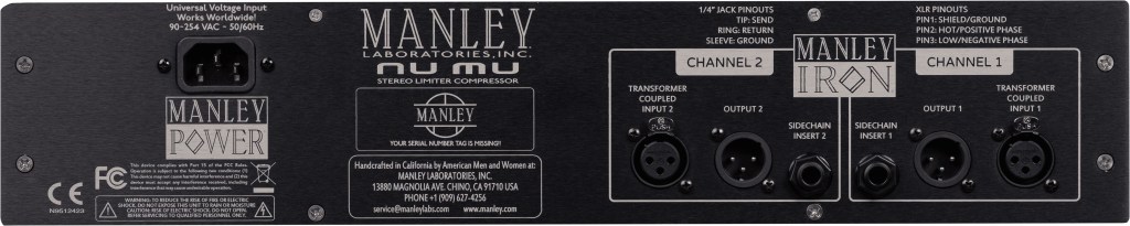
The unit features a 100 Hz high-pass filter with a 6dB per octave slope for internal signal detection, while also providing sidechain send/return inserts for external processing.

When the sidechain send/return inserts are connected, the internal detection circuit is bypassed, and the unit derives its detection exclusively from the external sidechain signal.

Therefore, a simple EQ connection is recommended for this function. To facilitate this, I am currently seeking a cheap used 1U rackmount EQ (like the Behringer FBQ1502HD) to utilize specifically with this sidechain insert.


Final Thought

It’s really great gear! I think it can be used in three ways:

  1. As a saturator: Running signals through the Manley Nu Mu without any gain reduction.
  2. For characteristic grooves: Using the sidechain function to create unique grooves with rhythmic signals.
  3. As a bus compressor: Using it for mixing or mastering.

I’ll be writing a follow-up post once I acquire an EQ or stereo imaging hardware for my setup. Thanks for reading! See you in the next post.

DIY Audio Project #1 | Tube Saturator with Baxandall EQ (Part 3): Design and Order PCB Circuit

Hello, I’m Jooyoung Kim — an audio engineer and music producer.

Lately, I’ve been so tied up with outside commitments that I feel like I’ve neglected my own music projects. After visiting the exhibition by artists Chungha Ester Lim and Inguen Nam last time, I found myself reflecting quite a bit. Today, I went back again to see the works and reset my mindset.

I’m juggling a lot of different things, so time is always tight—but even if I have to carve it out little by little, I need to make it happen. The same goes for this blog.

Anyway, today’s post continues from the previous one and focuses on the PCB fabrication process.

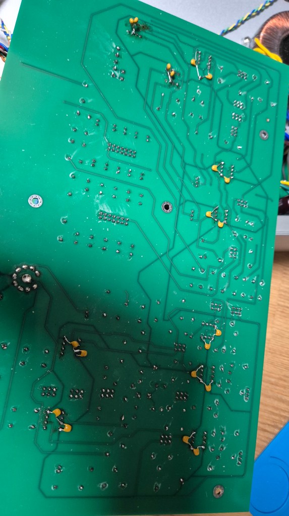
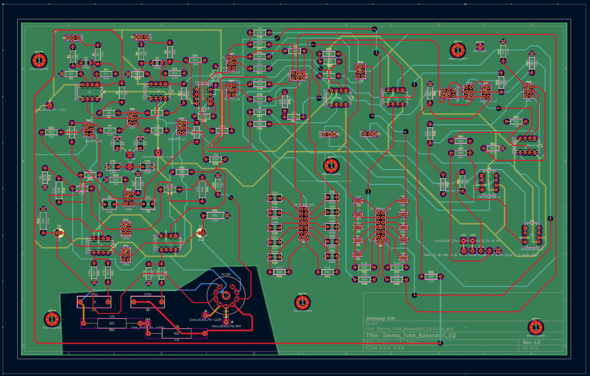
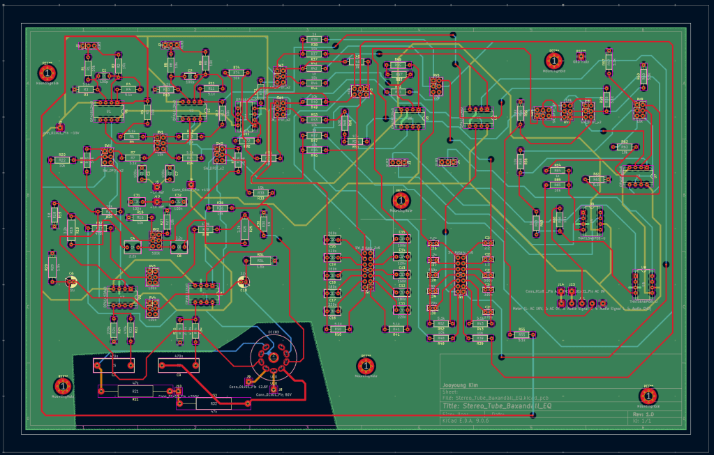
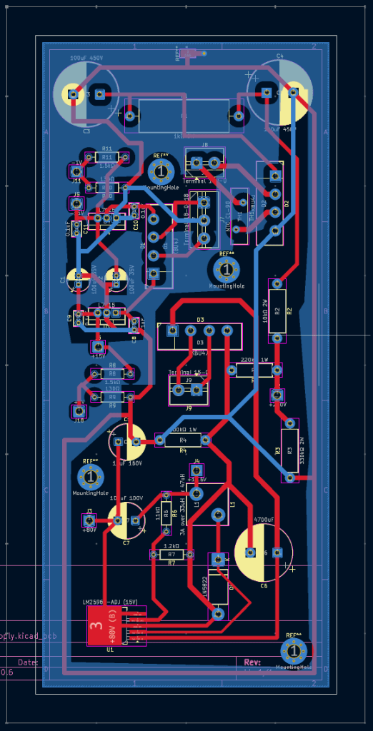
Once the schematic design is complete, the next step is translating it into a PCB layout. At its most basic, a PCB consists of two layers: the first layer carries the signal traces, and the second layer serves as ground. However, in audio equipment with a high component count, two layers may not be sufficient. In my case, I had to distribute multiple DC voltage rails throughout the circuit, and several chips had many pins that required careful routing. As a result, I designed the main board as a four-layer PCB, while the power supply board remained a two-layer design.

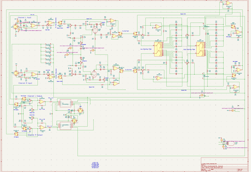
The issue—if I didn’t mention this in the previous post—is that even if everything looks perfect in the schematic, it doesn’t automatically translate cleanly onto the PCB.

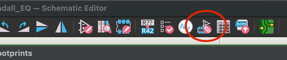
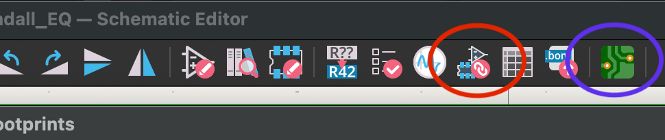
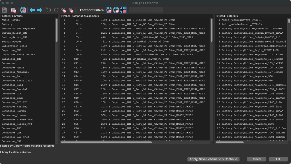
If you look at the top-right area of the schematic, you’ll see link indicators for the op-amps and IC chips. Clicking one of those opens a window where you have to manually assign the correct physical package for each component. This is called a footprint.

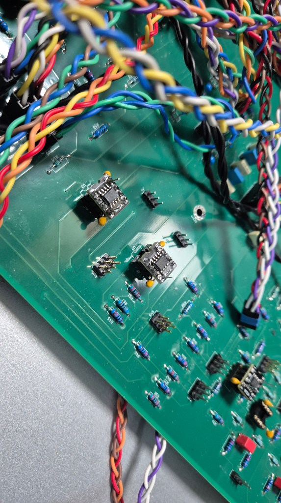
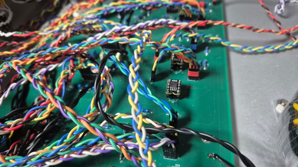
To assign the correct footprint, you need to carefully cross-check each part against its datasheet and match the exact specifications. Honestly, that process nearly drove me crazy. After soldering everything together, I discovered about three problematic spots. I managed to fix them with some creative rework, but since I also had to revise the EQ bypass section anyway, I ended up redesigning the PCB and placing a new order. The thought of desoldering everything and starting over again is… thrilling, to say the least.

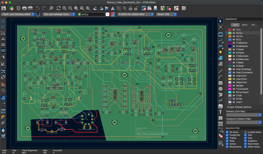
And even after that, you’re still not done. Once everything is set up, clicking the PCB editor icon opens the layout window.

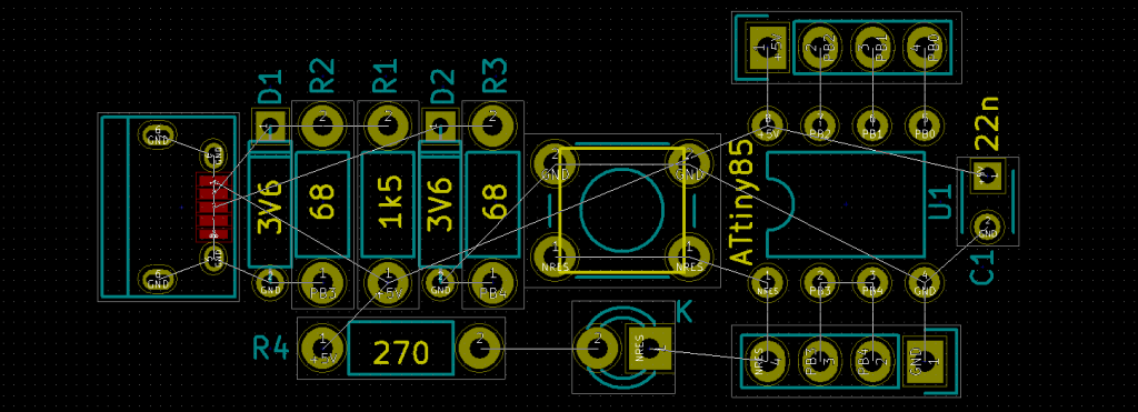
From there, you import all the assigned footprints. When they first load, they appear scattered randomly across the board.

I had around 150 components on the main board alone, so seeing them all clumped together at once was a bit overwhelming.

From that point on, it’s a lot of manual routing. For the ground plane, there’s no need to manually connect traces—filling the ground layer with copper automatically connects everything. For the power supply board, however, I kept it to two layers to reduce costs, so I cleared certain copper areas and routed the power traces manually. In the main board, I also removed copper around the high-voltage tube section to help minimize potential noise issues.

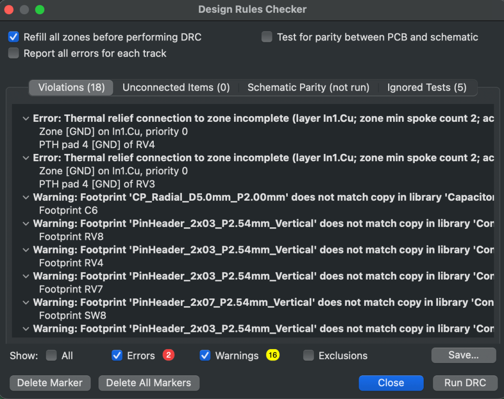
Once the layout is complete, you run a final design rule check. You’ll see a list of errors and warnings. If certain warnings are triggered by intentional design decisions, you can ignore them—but everything else should be reviewed carefully. In my case, I found a few unconnected traces that I had missed.

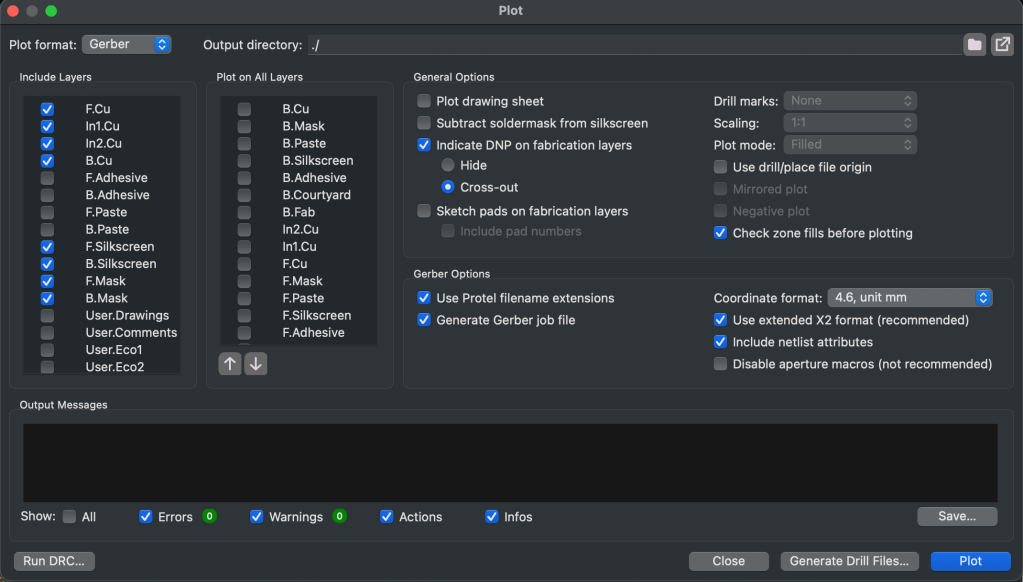
After that, you define the board outline using the Edge.Cuts layer. Then you go to File → Plot, select all the required layers, and generate the fabrication files. Since the plotted files don’t include drill data, you also need to export a separate drill file.

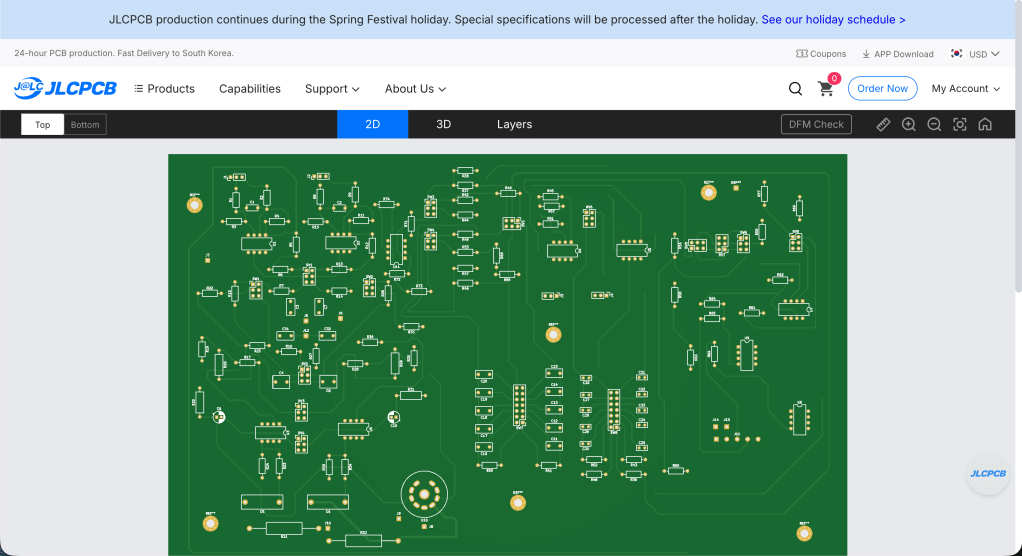
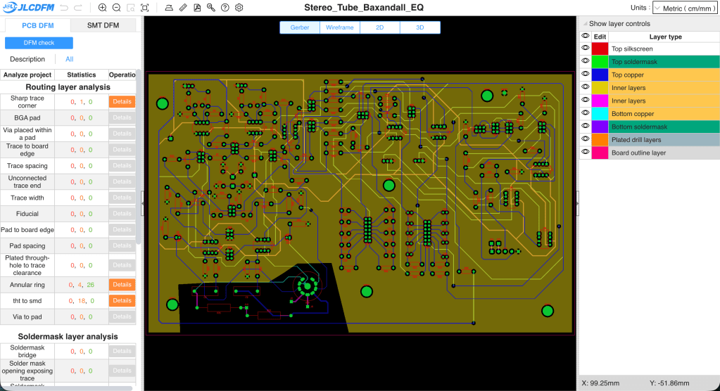
I ordered my PCBs from JLCPCB. After compressing all the generated files into a single ZIP archive and uploading it, you can preview the board before placing the order. There’s also a DFM (Design for Manufacturability) check that identifies potential production issues or design mistakes. It seems the manufacturer performs an additional review after you place the order as well.

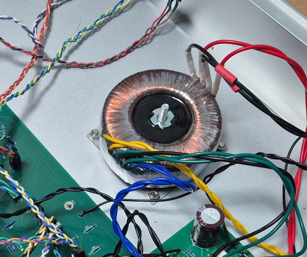
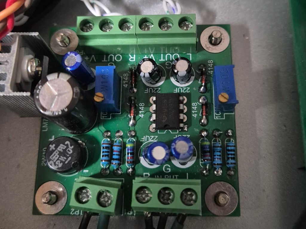
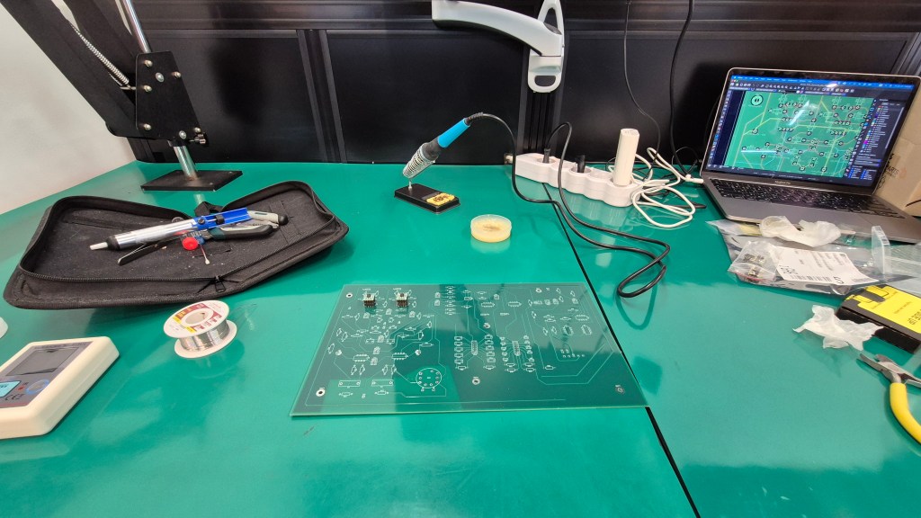
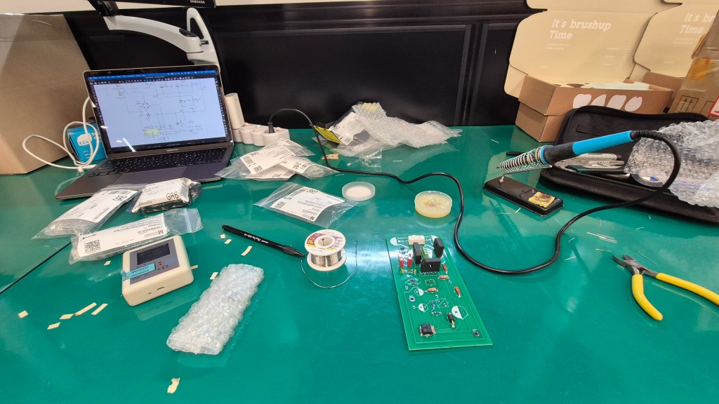
Once the boards arrive, all that’s left is soldering. For distributing multiple voltage rails, I had a custom toroidal transformer made. Since the design includes vacuum tubes, higher voltages are required—far beyond what a simple adapter can provide. Toroidal transformers also tend to be more resistant to ground-related noise.

In the next post, I’ll talk about the case fabrication and the final assembly process. I’ve already sent out the enclosure drawings, and since the PCB has been revised, the final installment may take a bit longer to publish. In the meantime, I’ll think about what topic to cover next.

See you in the next post!
DIY Audio Project #1 | Tube Saturator with Baxandall EQ (Part 2): Simulation

Hello, this is Jooyoung Kim — an audio engineer and music producer.

I ended up taking on way more classes than I expected this semester…
and honestly, just preparing for them is killing me. Haha. Every day feels like it disappears while I’m organizing lecture materials… 😢

And somehow, it’s already been almost two weeks…!

Today, following up on my previous post, I’d like to talk about running simulations.

Alright—let’s get started!


To run simulations in KiCad, you need a library file for each component.

The file extension is .lib.
As an example, here’s roughly what the library file looks like for a potentiometer (variable resistor) I created:

* Logarithmic Potentiometer Subcircuit (A-type taper)
.SUBCKT DUAL_POT_10K_LOG 1 2 3 4 5 6 SET=0.5 VALUE=10k
* Unit A (Log curve: 10% resistance at 50% rotation)
Ra1 1 2 {VALUE*(1-pow(10, -SET))+0.001}
Ra2 2 3 {VALUE*pow(10, -SET)+0.001}
* Unit B
Rb1 4 5 {VALUE*(1-pow(10, -SET))+0.001}
Rb2 5 6 {VALUE*pow(10, -SET)+0.001}
.ENDS

For components that are already built into KiCad, these libraries are applied automatically.

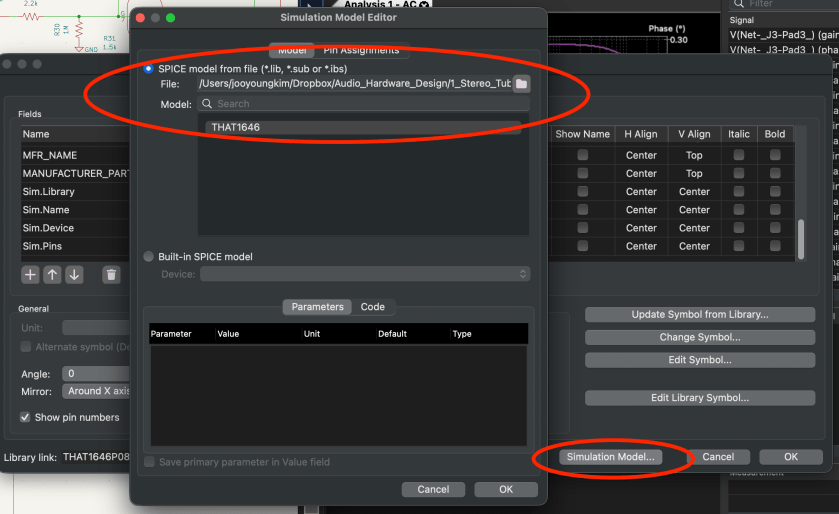
But for components that aren’t, you have to double-click the part, go to the component properties, click Simulation Model, and manually add everything… one by one.

Yeah… that part alone ate up a lot of time. 😅

For the audio output stage, you can simply exclude the XLR jack from the simulation. If you connect it to ground through a large resistor, you can still simulate the audio signal at the output.

Simulation isn’t exactly… simple.

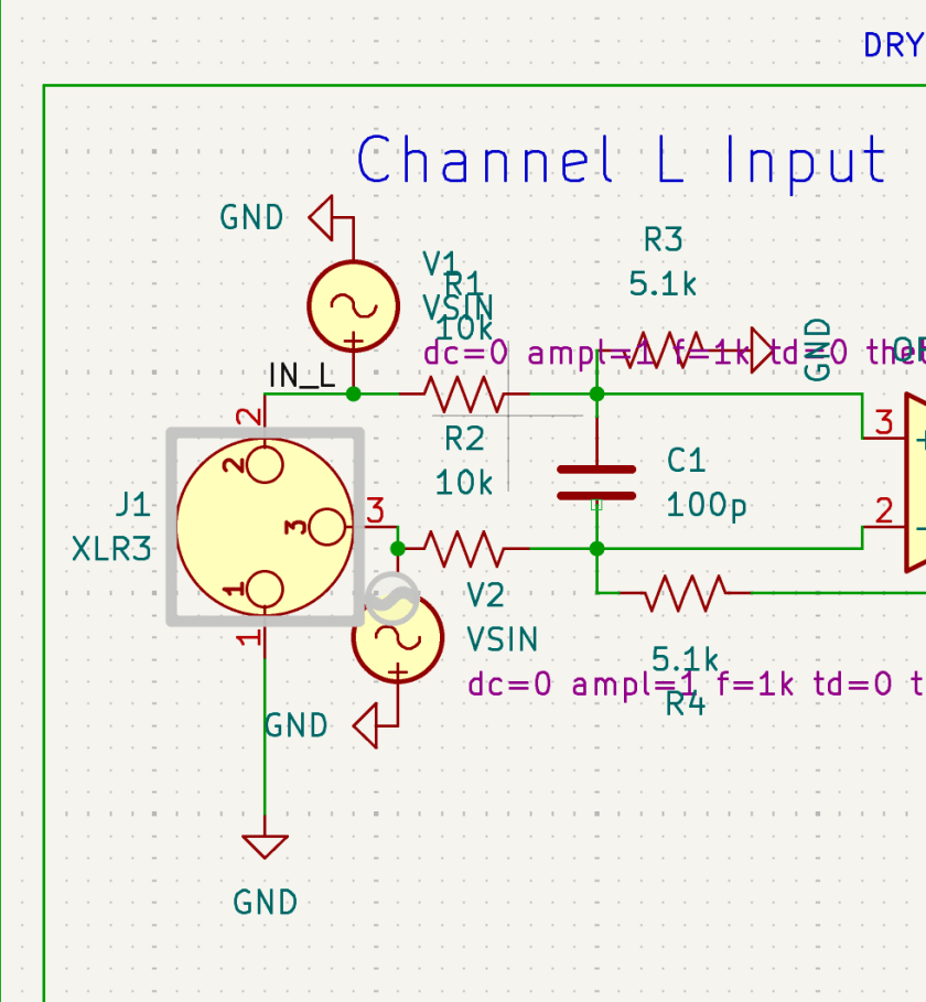
You need to supply DC where DC is required, and AC where AC is required. When checking frequency response and phase response, you’ll need to apply an AC sine signal to both the hot and cold sides.

What’s especially annoying is that every single pin must be connected. If even one pin is left floating, KiCad will keep throwing errors.

Personally, once the circuit is mostly finalized, I find it easier to copy it into a separate file and run simulations there.

Yes, you can exclude individual components from simulation, but…
if there’s an oscillator in the schematic, things get messy again when moving on to PCB layout. 😓

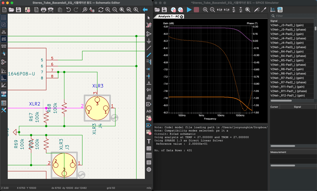
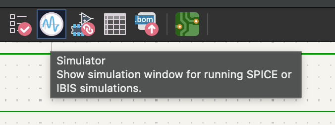
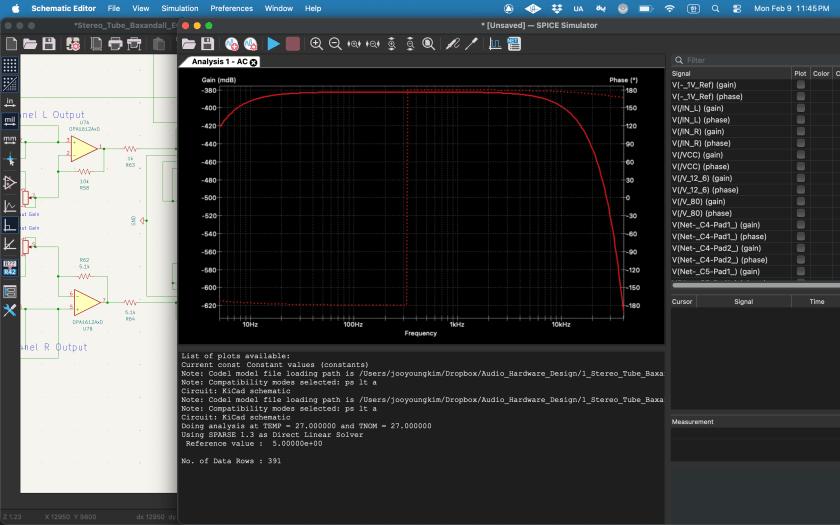
Anyway—once all the libraries are properly set up, you can click the oscillator-looking icon in the top-right corner. That will bring up the simulation window.

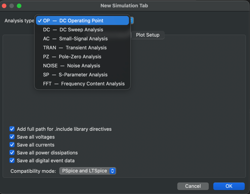
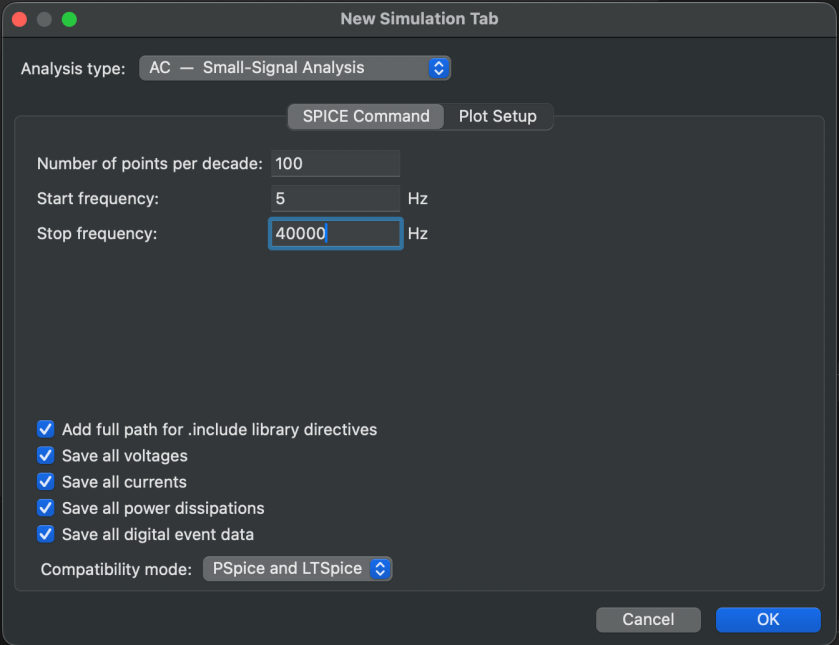
If you click the play button in the top-left, a settings window appears where you choose what and how you want to analyze.

Since we’ve attached an AC 1 V source to observe frequency and phase response,
we’ll select AC analysis. With just these settings, you can already see the response clearly.

Now, if playback actually works, it feels amazing. But realistically… it probably won’t work on the first try. (It definitely didn’t for me.) If it doesn’t run, something is disconnected, or a library is wrong—and you’re in for a lot of fixing.

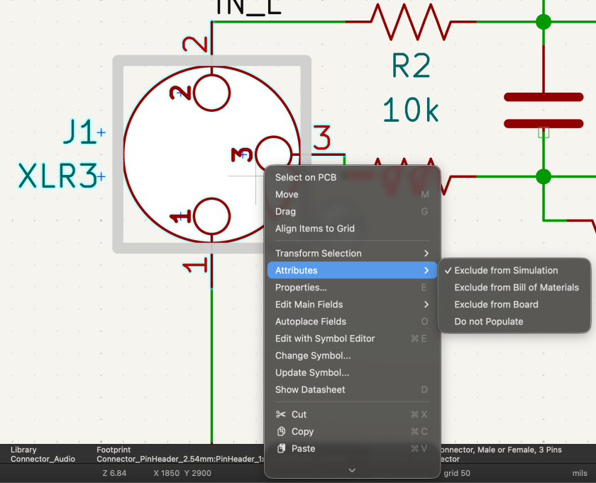
One important thing: if you’ve broken out pins separately for XLRs or DC/AC wiring, you must make sure they’re excluded from the simulation.

You can do this by right-clicking, then selecting Attribute → Exclude from Simulation. The same Attribute settings can also exclude things from board or component configurations.

Simulation is critically important—and you shouldn’t only check the final stage. Especially for processors with multiple stages, you need to verify that the signal behaves correctly at each step.

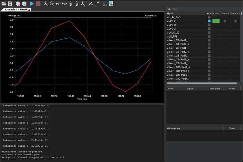
If impedance isn’t handled properly, the signal simply won’t flow the way you expect—and that will happen. Also, if you want to view signals in an oscillator-style analyzer, you’ll need to switch from AC analysis to Transient analysis.

This is also a convenient place to check for phase inversion.

And if you see signals that don’t line up properly here… welcome to modification hell. 😄 While running simulations to write this blog post… I literally just realized a major mistake.

I already ordered the PCB and finished soldering everything… so yeah, I’m screwed. Haha.

Resistor values are easy enough to change, but everything else was fine—until I noticed that bypassing the EQ flips the phase… and I only realized this now. 😭😭

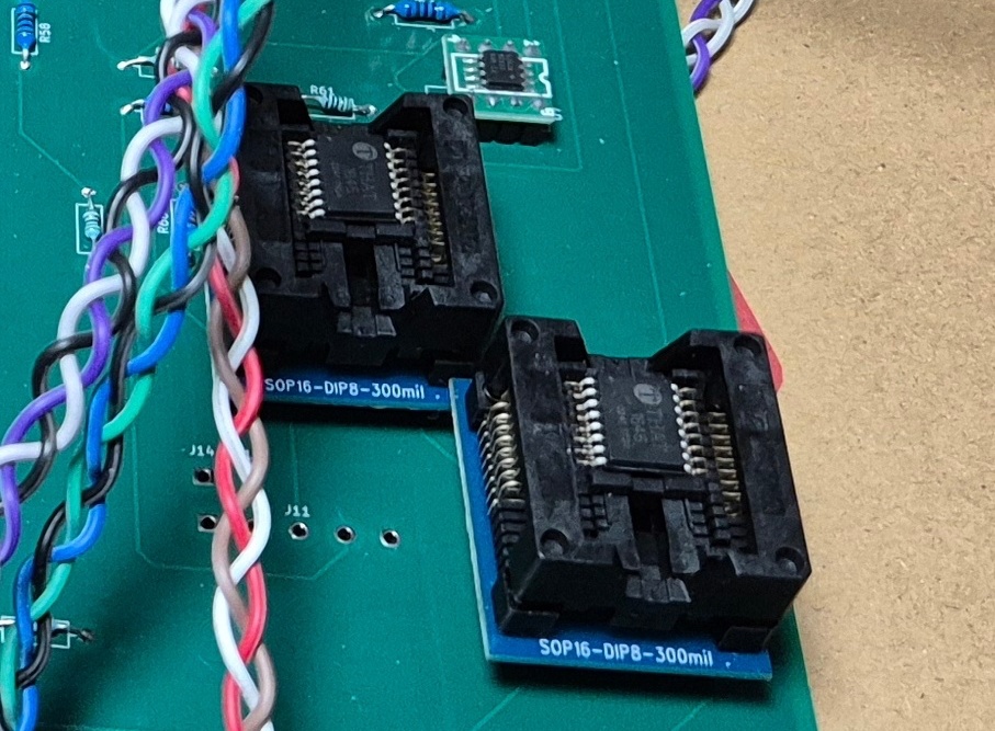
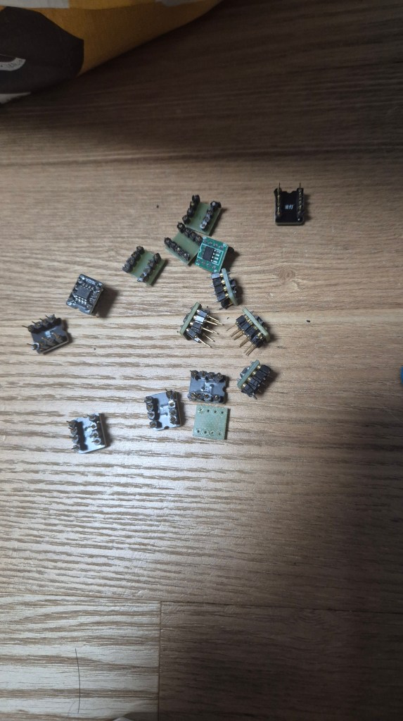
The final THAT chip is a 16-pin device, but I used an 8-pin footprint and bought an adapter socket. Unfortunately, I placed two of them way too close together, so I’ll probably have to desolder and reposition them.

Including the power section, there must be around 180 components total… I’ll likely have to order a separate Ver.2 PCB later and migrate everything over. 😢

Anyway—this is exactly why simulation matters.

One more important thing: in simulations, op-amps are assumed to be ideal. Because of that, in Transient analysis, you won’t see distortion even at maximum dB levels. You need to keep this limitation in mind when interpreting results.

After all that, it’s time to move on to PCB design.

Apparently, this is often called “art” or “artwork.”

And honestly… there’s no grind quite like this kind of grind. If I include PCB layout as well, this post will get way too long, so I’ll wrap things up here for today.

See you again in the next post! 😊
DIY Audio Project #1 | Tube Saturator with Baxandall EQ (Part 1): Concept and Implementation in Digital

Hi! This is Jooyoung Kim, a mixing engineer and music producer. In the previous post, ‘Wrapping Up 2025‘, I mentioned that I was developing circuits for my personal audio hardware.

Now that the circuit design and simulation are finished and the components and PCBs have been ordered, I am writing this post to record the process—including the failures and successes along the way. To be honest, since the build isn’t finished yet, I can’t guarantee it will be a 100% success.

However, I thought it would be a great opportunity to share what is actually needed for the design process, starting from scratch. I want to explain things in a way that anyone, even those with zero prior knowledge, can easily follow along.

Let’s start!

Concepts

I really love the analog “tube” sounds. However, I don’t have any stereo tube saturator hardware. Also, I don’t have an EQ that can be used for mastering either.

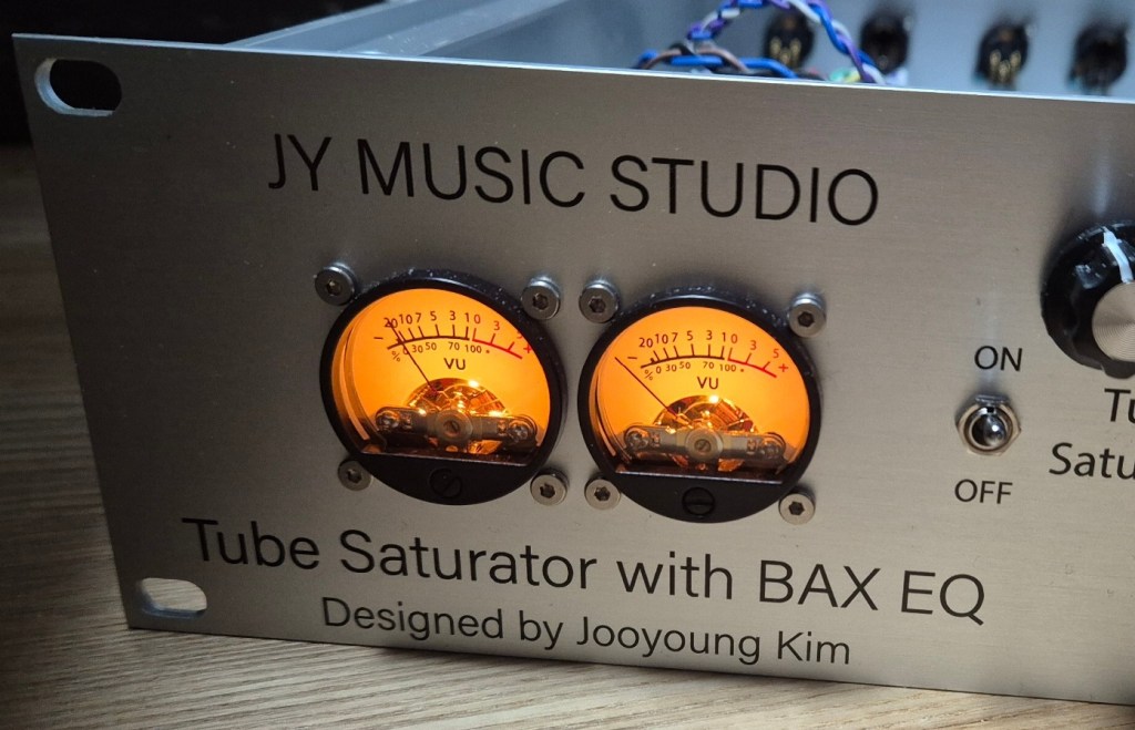
Therefore, I decided to make a stereo tube saturator with Baxandall EQ!
I used KiCad for this project. I highly recommend it because it allows you to seamlessly transition from circuit design to simulation, and finally to PCB layout. But that also means… once you’re done with the circuit, you still have two massive tasks waiting for you (hahaha…). I honestly had no idea what I was getting into until I finished the initial design!


Tube Parts

I already have two tubes (JJ Electronics’ ECC83) that were replaced from my Stam Audio SA-2A, so I wanted to use them for this project. Since I intend to use this gear in the mastering process, I decided to use just a single tube to drive the gain after the input stage.

I also designed the tube stage with adjustable ‘ASYMMETRY’ and ‘DENSITY’ parameters.

ASYMMETRY (Bias Adjustment) parameter controls the grid bias (+/-1V spans in my circuit)) of the vacuum tube. By shifting the bias point, it allows the waveform to clip asymmetrically, which generates even-order harmonics.

DENSITY (Saturation & Body) parameter adjusts the amount of feedback at the cathode stage. By controlling the effectiveness of the bypass capacitor, it pushes the tube to hit its saturation point harder or softer.

To develop this parts, I utilized Gemini (the free version) and referenced the manual of the Wave Arts Tube Saturator Vintage plugin for inspiration. Even though I majored in physics, it’s a field of pure science focused on fundamental principles, so I didn’t really cover practical applications like circuit design. As I mentioned, I actually had very little in-depth knowledge of electronic circuits starting out. But those tools were a huge help! Seriously, use AI tools—they can bridge the gap!


Baxandall EQ Parts

The EQ design is straightforward, consisting of two sections: Low and High. While the gain is continuously adjustable, I made the frequency switchable using rotary switches, allowing for precise and repeatable settings.

Baxandall EQ circuits are quite simple and well-documented, so you can easily find various schematics online to use as a reference.


Input & Output Parts

The input stage was simple enough, but the output stage was a total ambush. I wanted to include a Mix knob, a Mix Bypass switch, a Total Bypass switch, and an Output Gain knob. Trying to integrate all these features into the signal path turned into a bit of a mess!

After completing the overall design, I realized a crucial detail: every single stage had to be in the same phase! If the phases didn’t match, the Mix knob would be useless. So, I had to go back and triple-check the phase of every section after all the work was seemingly ‘done.’ I’ll talk more about this in my next post about the simulation process.


Power Parts

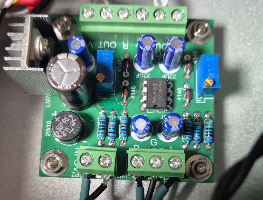
To ensure this hardware works in various environments, I included an adjustable voltage switch(220V-110V) in the power circuit. Since the design requires multiple voltage rails—250V, ±15V, +80V, +12.6V, and ±1V—I had to use a complex, custom-spec toroidal transformer. Managing all these different power requirements in one unit was quite a challenge!

Heat dissipation was a major concern for this build. I basically tortured Gemini with endless questions, forcing it to crunch the numbers until I was sure every component could handle the thermal load.

I’d like to dive deeper into the phase issues and buffers that need to be considered in the simulation, but it would make this post way too long. So, I’ll cover those in the next one.

See you then!